What a transmitter is, and why it sends 4–20 mA

A control room operator looks at a screen showing a tank is 62% full and running at 84 °C. They are not looking at the tank. They are looking at numbers produced by two field devices called transmitters, and the reliability of everything that follows depends on those two devices being right.

What a transmitter does

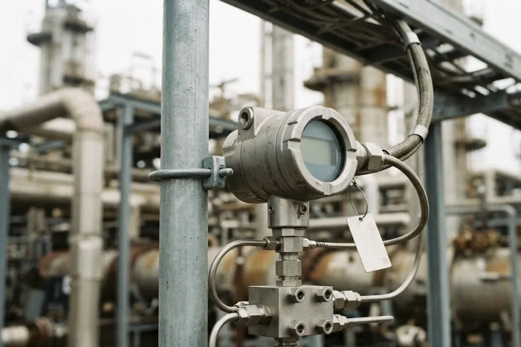
A transmitter has one job: turn a physical quantity into a standard signal that a control system can read.

It has three parts:

1. The sensor — the part physically exposed to the process. A diaphragm that flexes with pressure, a platinum element whose resistance changes with temperature, a radar antenna.
2. The transducer — converts that physical change into a small electrical signal.
3. The transmitter electronics — amplify, linearise, compensate for temperature, apply the configured range and drive the output signal.

The word transmitter strictly means only the third part, but in the field it means the whole assembly, and the tag number on the drawing refers to that.

Why 4–20 mA

For sixty years the standard analogue instrument signal has been a current loop where 4 mA represents 0% of range and 20 mA represents 100%. Four design decisions are packed into that choice, and each one is worth understanding.

Current, not voltage

A voltage signal drops over the length of a cable. Run 300 metres from a field transmitter to a marshalling cabinet and the voltage at the far end is not the voltage that was sent. Current in a series loop is the same everywhere. Cable resistance, within limits, changes nothing. That single property is why current won.

Live zero

If the signal ran 0–20 mA, then a reading of 0 mA would be ambiguous: the process might genuinely be at zero, or the wire might be broken. Starting at 4 mA removes the ambiguity — 0 mA can only mean a fault.

Two wires do everything

A 4–20 mA transmitter draws its power from the same two wires that carry its signal. The device needs less than 4 mA to run, which is exactly why the live zero sits there. Two wires instead of four, across thousands of instruments, is a large saving in cable, tray and termination.

It suits intrinsic safety

The energy in a 24 V, 20 mA loop is small enough to be made intrinsically safe with a barrier, which is what allows instruments in Zone 0 and Zone 1 without flameproof housings.

Converting between mA and engineering units

percent = (mA − 4) / 16
value   = LRV + percent × (URV − LRV)

Where LRV and URV are the lower and upper range values the transmitter is configured to. For a transmitter ranged 0–10 bar reading 12 mA: (12−4)/16 = 0.5, so 5 bar. You will do this arithmetic constantly during commissioning.

HART: digital data on the same wires

HART superimposes a small digital signal on top of the 4–20 mA current without disturbing it. The analogue value continues to drive the control system while the digital layer carries device tag, configuration, diagnostics and additional variables.

This is why a technician can stand at a transmitter with a handheld communicator, read its serial number, change its range and run a self-test — all without disconnecting anything or disturbing the loop. Most transmitters sold today are HART-capable whether or not the project uses it.

Fieldbus protocols (FOUNDATION Fieldbus, PROFIBUS PA) go further and make the signal fully digital with multiple devices per pair, but 4–20 mA with HART remains the most common arrangement by a wide margin.

Choosing a measurement principle

Most instrumentation work is selection, not invention. The table below is the shape of that decision.

Filter Process measurement principles and where each fits

10 rows

Variable	Principle	Typical accuracy	Good for	Watch out for
Pressure	Piezoresistive / capacitive diaphragm	±0.04 – 0.1% span	Almost all gauge and differential pressure duties	Impulse line blockage, freezing and trapped gas giving false readings
Temperature	RTD (Pt100)	±0.1 – 0.5 °C	Process temperatures below about 600 °C where accuracy matters	Lead resistance — always use 3- or 4-wire; thermowell insertion depth
Temperature	Thermocouple (K, J, N)	±1 – 2 °C	High temperature, furnaces, fast response, rugged duty	Cold junction compensation and correct extension cable polarity
Flow	Differential pressure (orifice plate)	±1 – 2% rate	Clean gas, steam and liquid. Cheap, universal, well understood	Permanent pressure loss; narrow turndown of about 3:1
Flow	Magnetic (magmeter)	±0.2 – 0.5% rate	Conductive liquids, slurries, no pressure drop, full bore	Will not work on hydrocarbons or any non-conductive fluid
Flow	Coriolis	±0.1% rate	Direct mass flow and density. Custody transfer and dosing	Cost, size and sensitivity to external pipe vibration
Flow	Vortex shedding	±0.75 – 1.5% rate	Steam and clean gas, no moving parts	Needs minimum velocity — reads nothing at low flow
Level	Differential pressure / hydrostatic	±0.5% span	Vessels with stable, known density	Density change or foam directly falsifies the reading
Level	Guided wave radar	±2 – 5 mm	Most liquids, unaffected by density, pressure or temperature	Probe coating in sticky service; interface detection needs care
Level	Ultrasonic (non-contact)	±3 – 6 mm	Open tanks, sumps, water service, no process contact	Vapour, foam and heavy dust absorb the signal

No measurement principle is universally best. The selection is driven by the fluid, the accuracy the process actually needs, whether the line can be broken into, and what the plant already stocks as spares.

The selection rarely comes down to accuracy alone. In practice it is:

1. Will it work in this fluid at all? A magmeter in a hydrocarbon line is not a poor choice, it is a non-functional one.
2. What accuracy does the process actually need? A 0.1% Coriolis meter on a line where ±5% would do is money spent for nothing.
3. Can the line be broken into? Retrofitting an in-line meter means a shutdown; a clamp-on ultrasonic does not.
4. What does the plant already stock? Standardising on fewer models means fewer spares and technicians who already know the menus.

Tag numbers and how to read a loop

Every instrument has a tag from ISA 5.1, such as PT-1024:

• First letter — the measured variable: P pressure, T temperature, F flow, L level, A analysis.
• Following letters — the function: T transmitter, I indicator, C controller, V valve, S switch, AH/AL alarm high/low.
• Number — the loop, usually carrying the unit or area number.

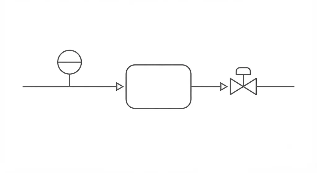
So a complete control loop reads as a sentence: PT-1024 measures the pressure and sends 4–20 mA to PIC-1024, the controller, which compares it against setpoint and sends its own 4–20 mA output to PV-1024, the control valve. Same number, one loop, four documents describing it — the P&ID, the loop diagram, the hook-up drawing and the instrument datasheet.

What to take away

• A transmitter converts a physical quantity into a standard signal; the sensor is the part that touches the process.
• 4–20 mA survives because current is immune to cable resistance, the live zero makes a broken wire unmistakable, two wires carry both power and signal, and the energy is low enough to be intrinsically safe.
• percent = (mA − 4) / 16. Learn it.
• HART adds digital diagnostics and configuration without disturbing the analogue value.
• Select a measurement principle on whether it works in the fluid first, accuracy second.
• Ranging is configuration; calibration is verification. They are different activities.